
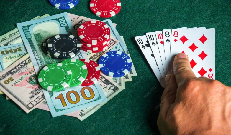
₹100 to ₹10,000: What the Math Says About Compounding Bets
Start with ₹100.
Win.
Put the entire amount into the next round.
Win again.
Repeat.
On paper, the numbers can become exciting very quickly:
₹100 → ₹200 → ₹400 → ₹800 → ₹1,600 → ₹3,200 → ₹6,400 → ₹12,800
Only seven successful rounds.
₹100 has apparently become more than ₹10,000.
At first glance, this can make compounding look like a shortcut:
“Bas 7 rounds continuously sahi chahiye.”
But this way of looking at the sequence focuses entirely on how quickly the amount grows.
It ignores the other side of the calculation:
How quickly does the probability of completing the entire sequence shrink?
That is where the mathematics becomes much more interesting.
This article does not provide a staking system or recommendation. Instead, we’ll use hypothetical examples to understand exponential growth, consecutive-event probability, payout ratios and why turning ₹100 into ₹10,000 is mathematically very different from simply multiplying ₹100 by 100.
First, What Does “Compounding” Mean Here?
In finance, compounding usually refers to returns being added to principal so that future returns can themselves generate returns.
For example, if ₹100 grows by 10%, it becomes:
₹110.
If the next 10% is calculated on ₹110 rather than the original ₹100, the amount becomes:
₹121.
The return itself has started participating in future growth.
A similar-looking idea is sometimes applied to game outcomes:
start with one amount, add the gain, and expose the enlarged amount to another uncertain round.
Mathematically, however, this has an important consequence.
Your potential amount grows.
But so does the amount exposed to the next uncertain outcome.
A Simple Hypothetical Doubling Model
Because “777 Game” can refer to different formats, we will not assume that any particular platform actually offers a 2x return or 50/50 outcomes.
Instead, consider a fictional mathematical experiment.
Assume:
- Starting amount = ₹100
- Successful round doubles the total amount
- Unsuccessful round loses the amount exposed in that round
- Probability of success on each independent round = 50%
Again, this is an illustrative probability model, not a description of a specific 777 platform.
How Many Doublings Turn ₹100 Into More Than ₹10,000?
Let’s calculate.
Starting amount:
₹100
After 1 successful round:
₹200
After 2:
₹400
After 3:
₹800
After 4:
₹1,600
After 5:
₹3,200
After 6:
₹6,400
After 7:
₹12,800
So under this fictional doubling model, seven consecutive successful rounds would take ₹100 past ₹10,000.
The Growth Looks Extraordinary
The general formula is:
Final Amount = Starting Amount × 2n
where n is the number of consecutive successful doublings.
For seven:
₹100 × 27
= ₹100 × 128
= ₹12,800.
This is exponential growth.
Each additional successful round has a larger financial effect than the previous one because the amount being doubled has increased.
But Now Calculate the Other Exponential
If each independent round has a 50% probability of success, the probability of seven consecutive successes is:
(0.5)7
= 1/128
= 0.78125%
So the same exponent that makes the amount grow rapidly also makes the probability of completing the entire sequence shrink rapidly.
This creates a useful symmetry:
Amount multiplier after 7 wins = 128
Probability of 7 consecutive wins = 1/128
under the hypothetical fair doubling model.
₹12,800 Looks Different When Paired With 0.78125%
If you look only at the amount:
₹100 → ₹12,800
sounds remarkable.
If you look only at the probability:
1 chance in 128
sounds very different.
A proper mathematical analysis has to look at both.
Potential return without probability is incomplete information.
Let’s Put Both Sides in One Table
| Consecutive Successful Rounds | Hypothetical Amount | Probability of Completing Sequence at 50% Per Round |
|---|---|---|
| 0 | ₹100 | 100% |
| 1 | ₹200 | 50% |
| 2 | ₹400 | 25% |
| 3 | ₹800 | 12.5% |
| 4 | ₹1,600 | 6.25% |
| 5 | ₹3,200 | 3.125% |
| 6 | ₹6,400 | 1.5625% |
| 7 | ₹12,800 | 0.78125% |
This table shows something that a simple “₹100 to ₹10,000” screenshot usually doesn’t.
The amount and the probability are moving in opposite directions.
Why Doesn’t Compounding Improve the Probability?
Suppose the first round is successful.
Your hypothetical amount becomes:
₹200.
Has the probability of succeeding on round two increased?
Under our independent model:
No.
It remains:
50%.
After two successes, your amount becomes ₹400.
Does round three become easier?
Again:
No.
The amount has changed.
The assumed probability has not.
Money and Probability Are Different Variables
This distinction is fundamental.
Suppose you expose:
₹100
to a hypothetical 50/50 event.
Probability of success:
50%.
Now expose:
₹10,000
to the same event.
Probability of success:
still 50%.
The financial consequence has increased by 100 times.
The probability hasn’t changed at all.
Compounding Changes Exposure, Not the Outcome Generator
If a round’s outcome is independent of the amount involved, increasing the amount cannot make the preferred result more likely.
The generator does not mathematically care whether the amount is:
₹100
or:
₹6,400.
Under our simplified model, only the financial consequence changes.
The Most Dangerous Point Comes Near the End
Consider the sequence again:
₹100 → ₹200 → ₹400 → ₹800 → ₹1,600 → ₹3,200 → ₹6,400 → ₹12,800
After six consecutive successful rounds, the hypothetical amount is:
₹6,400.
Only one more successful round is needed to cross ₹10,000.
Psychologically, that can feel like:
“Itna aa gaya. Bas ek aur.”
But mathematically, if the next round remains 50/50, that final round still has:
50% probability of success
and:
50% probability of failure.
The previous six successes do not make the seventh easier.
The Final Round Risks Much More Than the First
At the beginning, the exposed amount was:
₹100.
Before the seventh hypothetical doubling, the amount is:
₹6,400.
The probability may be identical.
But the amount at risk is dramatically different.
This is one of the defining characteristics of full compounding.
One Failure Can Erase the Entire Chain
Under the all-in fictional example, imagine this sequence:
Win → Win → Win → Win → Win → Win → Loss
Six successful rounds occurred.
Accuracy:
6 out of 7 ≈ 85.7%.
That sounds excellent.
Yet if the entire accumulated amount was exposed every time, the final result of the chain is:
₹0.
This demonstrates why percentage of successful rounds alone does not describe the financial outcome of a compounding sequence.
85.7% Correct Can Still End at Zero
This is counterintuitive.
Someone might say:
“I was right six times and wrong only once.”
True.
But the one unsuccessful round occurred when the largest amount was exposed.
Therefore, the order of outcomes matters enormously when exposure changes between rounds.
Compare Two Seven-Round Sequences
Sequence A
Loss → Win → Win → Win → Win → Win → Win
Sequence B
Win → Win → Win → Win → Win → Win → Loss
Both contain:
6 wins and 1 loss.
Same success rate:
85.7%.
But under a strategy where the entire accumulated amount is repeatedly exposed, the financial paths can be radically different.
Outcome order matters because the amount changes over time.
This Is Called Path Dependence
A process is path-dependent when the route taken affects the final result, not merely the total number of successful and unsuccessful events.
Compounding creates strong path dependence.
A failure early in the sequence and a failure late in the sequence can have very different financial consequences.
Now Change the Success Probability to 60%
Suppose, purely hypothetically, each independent round has:
60% probability of success.
Probability of seven consecutive successes:
0.67
≈ 0.02799
or:
≈ 2.80%.
That’s much higher than the 0.78125% probability under a 50% model.
But it is still far below 60%.
A High Single-Round Accuracy Can Become a Low Sequence Probability
This is one of the biggest lessons in compounding mathematics.
Suppose a predictor really had:
70% probability of success per independent round.
That sounds extremely strong.
But seven consecutive successes would have probability:
0.77
≈ 8.24%.
So even with a hypothetical 70% per-round success probability, completing seven straight successes would occur only about 8.24% of the time under the independence assumption.
What About 80% Accuracy?
Seven consecutive successes:
0.87
≈ 20.97%.
Even at a very high hypothetical 80% success probability, the probability of completing all seven rounds is only about:
1 in 4.77.
Again, a high probability for one event should not be confused with a high probability of a long uninterrupted sequence.
Compare Different Per-Round Probabilities
| Hypothetical Per-Round Success Probability | Probability of 7 Consecutive Successes |
|---|---|
| 40% | 0.164% |
| 50% | 0.781% |
| 60% | 2.799% |
| 70% | 8.235% |
| 80% | 20.972% |
| 90% | 47.830% |
This table illustrates why:
“My prediction is usually correct”
and:
“I can complete a long compounding chain”
are not equivalent claims.
Why Seven Consecutive Events Are So Demanding
For the entire chain to succeed:
Round 1 must succeed
AND Round 2 must succeed
AND Round 3 must succeed
AND Round 4 must succeed
AND Round 5 must succeed
AND Round 6 must succeed
AND Round 7 must succeed.
Every condition has to be satisfied.
Under independence, their probabilities multiply.
The Word “AND” Is Mathematically Expensive
Compare:
“Win at least one of seven rounds”
with:
“Win all seven rounds.”
These are completely different events.
Under a 50/50 independent model:
Probability of all seven successes:
1/128 ≈ 0.78125%.
Probability of at least one success in seven rounds:
1 – (0.5)7
= 127/128
≈ 99.21875%.
Same seven rounds.
Completely different probability question.
Compounding Requires the Harder Event
If the entire amount is repeatedly carried forward and one failure ends the chain, the relevant event is:
success AND success AND success AND success…
not:
at least one success.
This is why compounding targets can look easy when viewed as multiplication but difficult when viewed as probability.
₹100 to ₹10,000 Is a 100x Target
Ignoring the exact payout structure for a moment, increasing:
₹100
to:
₹10,000
requires multiplying the original amount by:
100.
That is a:
9,900% increase over the starting amount.
Any claim suggesting this can be achieved routinely should therefore be examined alongside the probability and risk required to generate such growth.
What If Each Success Adds Only 90% Instead of Doubling?
Now consider a different hypothetical payout.
Suppose a successful round turns ₹100 into:
₹190
rather than ₹200.
Each successful round multiplies the amount by:
1.9.
The formula becomes:
Final Amount = ₹100 × 1.9n
How Many Consecutive Successes Are Needed?
Let’s follow the approximate progression:
₹100
₹190
₹361
₹685.90
₹1,303.21
₹2,476.10
₹4,704.59
₹8,938.72
₹16,983.56
Now eight consecutive successful rounds are required to move beyond ₹10,000.
At 50% Per Round, Eight Consecutive Successes Have Probability
(0.5)8
= 1/256
≈ 0.390625%.
Reducing the payout multiplier increases the number of consecutive successes needed.
That can dramatically reduce the probability of completing the full chain.
Payout Structure Matters as Much as Win Probability
A statement such as:
“The result is 50/50”
does not tell us whether the financial proposition is mathematically fair.
We also need to know what happens financially after:
- A successful result
- An unsuccessful result
- Any special outcome
- Any fee or deduction
Probability and payout must be analysed together.
A 50% Chance With a 90% Net Gain Has Negative Expected Value
Consider a hypothetical ₹100 proposition:
- 50% probability: gain ₹90
- 50% probability: lose ₹100
Expected value:
(0.5 × ₹90) + (0.5 × -₹100)
= ₹45 – ₹50
= -₹5.
So the expected result is:
-₹5 per ₹100 exposure
under that hypothetical model.
Compounding Does Not Remove Negative Expected Value
This is critical.
If the underlying proposition has a mathematical disadvantage, repeatedly multiplying the amount after successful rounds does not change the underlying probability/payout relationship into a positive one.
It changes the distribution of possible financial outcomes.
It does not magically repair the expectation.
Expected Value and “Chance of Reaching ₹10,000” Are Different Questions
Expected value asks:
What is the probability-weighted average result across repeated comparable experiments?
Target probability asks:
What is the chance that this particular sequence reaches a specified amount before failing?
These should not be confused.
What If You Stop Before ₹10,000?
Now we have a different mathematical experiment.
Suppose someone stops after:
3 consecutive successful rounds.
Under the hypothetical doubling model:
₹100 → ₹200 → ₹400 → ₹800.
Probability of completing three independent 50% successes:
(0.5)3 = 12.5%.
This is much higher than the:
0.78125%
probability of completing seven.
But the target amount is also much smaller.
This illustrates a general trade-off:
Requiring a longer uninterrupted sequence can increase the possible terminal amount while reducing the probability of reaching it.
There Is No Free Exponential Growth
Whenever a hypothetical amount grows exponentially through repeated uncertain events, ask what is happening to the probability of completing the required sequence.
If each stage has probability less than 100%, requiring more consecutive successful stages usually reduces completion probability.
The attractive growth curve tells only half the story.
Why Social Media Examples Can Be Misleading
Imagine seeing a screenshot:
₹100 → ₹200 → ₹400 → ₹800 → ₹1,600 → ₹3,200 → ₹6,400 → ₹12,800
The screenshot shows one successful path.
It does not show how many unsuccessful paths existed before it.
Suppose 128 independent people each attempted the hypothetical seven-round 50/50 sequence once.
The expected number completing all seven would be:
128 × 1/128 = 1.
That one successful person’s screenshot could become highly visible.
The other 127 attempts might never be posted.
This Is Survivorship Bias
Survivorship bias occurs when successful cases are highly visible while failed cases disappear from observation.
Suppose thousands of people try an aggressive compounding challenge.
A small number reach a dramatic target.
Those successful sequences are shared:
“₹100 se ₹12,800!”
But without knowing how many total attempts occurred, the screenshot tells us almost nothing about the probability of reproducing the result.
One Winner Does Not Tell You the Success Rate
Imagine seeing:
10 successful ₹100-to-₹10,000 examples.
Were there:
12 total attempts?
That would be extraordinary.
Or:
100,000 total attempts?
That would tell a completely different story.
The denominator matters.
Always Ask: “Out of How Many Attempts?”
This question is useful whenever dramatic compounding results are presented.
Not:
“How much did this person make?”
but:
“How many comparable attempts produced this outcome?”
A success story without the number of attempts cannot establish a reliable success probability.
Starting Over Changes the Probability Question
Suppose a seven-round chain fails.
Then someone starts again from ₹100.
Each new attempt creates another opportunity to complete seven consecutive successes.
That means the probability of succeeding at least once across multiple independent attempts is higher than the probability of succeeding in one attempt.
But more attempts also mean more starting amounts are exposed.
Example: Ten Independent Attempts
Under our hypothetical fair doubling model, probability of one complete seven-win chain is:
1/128.
Probability one attempt fails to complete it:
127/128.
If ten independent attempts are made, probability all ten fail is:
(127/128)10
Therefore, probability of at least one successful chain is:
1 – (127/128)10
which is approximately:
7.54%.
More Attempts Increase the Chance of Seeing One Success
This explains why rare-looking success stories eventually appear when enough attempts occur.
But this should not be interpreted as a recommendation to keep retrying.
The mathematical cost and expected outcome of repeated attempts must also be considered.
How Many ₹100 Attempts Are Being Exposed?
If each failed chain requires a fresh:
₹100
starting amount, then:
10 attempts = up to ₹1,000 in starting exposures.
100 attempts = up to ₹10,000.
So saying:
“Eventually one chain may work”
does not by itself establish profitability.
The total cost of all attempts matters.
A Fascinating Fair-Game Symmetry
Return to our simplified 50/50 fair doubling experiment.
One attempt starts with:
₹100.
Probability of reaching ₹12,800:
1/128.
Terminal amount if successful:
₹12,800.
Probability-weighted terminal value:
(1/128) × ₹12,800 = ₹100.
Under this idealized zero-cost model, the expected terminal value equals the original ₹100.
This is not a profit advantage.
It is simply another representation of a mathematically fair proposition.
The Distribution Has Changed Dramatically, Though
Even though the expected terminal value is ₹100 in that idealized example, the outcomes are extreme:
- Most chains finish at ₹0
- A small fraction finish at ₹12,800
This is completely different from simply keeping ₹100.
Same expected value does not mean same risk profile.
Expectation Does Not Describe Typical Experience
This is an important statistical lesson.
Suppose 128 hypothetical independent attempts are made.
Under the simplified model, we’d expect roughly one full seven-win chain on average.
That successful chain finishes at:
₹12,800.
The others finish at:
₹0
if every chain is all-in and stops at its first failure.
The average terminal amount can still work out around ₹100 per attempt in expectation.
But almost nobody experiences the average outcome of ₹100.
This Is Why Averages Can Hide Risk
Two systems can have identical expected values and completely different distributions.
One might produce:
₹90–₹110 almost every time.
Another might produce:
₹0 most of the time and ₹12,800 rarely.
The average alone does not describe the experience.
Now Introduce a Small Mathematical Disadvantage
Suppose success probability remains:
50%.
But instead of doubling, each successful round multiplies the total amount by:
1.9.
Now the payout is no longer perfectly matched to the 50/50 probability in our simplified example.
Repeated compounding does not eliminate this difference.
It compounds through the sequence too.
Small Differences Become Important Across Multiple Rounds
A 5% difference may look small for one round.
Across many multiplicative steps, differences accumulate.
This is why evaluating only:
“How often do I win?”
is insufficient.
You also need:
“How much is gained when successful compared with how much is lost when unsuccessful?”
Break-Even Probability Depends on the Payout
Suppose ₹100 is exposed.
A successful outcome gives a net gain of:
₹90.
An unsuccessful outcome loses:
₹100.
Let the break-even success probability be p.
Then:
90p – 100(1-p) = 0
Expand:
90p – 100 + 100p = 0
190p = 100
Therefore:
p = 100/190
≈ 52.63%.
So a 50% success rate would not be enough to break even under that hypothetical payout.
Winning Half the Rounds Can Still Lose Money
This is one of the most important conclusions.
Suppose over 100 identical ₹100 propositions:
50 succeed
50 fail.
Net gains:
50 × ₹90 = ₹4,500.
Losses:
50 × ₹100 = ₹5,000.
Overall:
-₹500.
Accuracy:
50%.
Financial result:
negative.
Compounding Cannot Be Evaluated From Accuracy Alone
Any serious mathematical analysis needs at least:
- Probability of each outcome
- Net gain after success
- Loss after failure
- Number of consecutive stages required
- Whether rounds are independent
- Any additional outcomes or deductions
Without these variables, statements such as:
“Seven wins can turn ₹100 into ₹10,000”
are mathematically incomplete.
What If You Remove Some Amount Along the Way?
Then it is no longer the same full-compounding experiment.
For example, if some amount is removed after successful rounds while only the remainder continues, the terminal-value distribution changes.
The amount exposed at each stage changes.
Therefore, the entire calculation must be rebuilt.
You cannot use the probability and payout calculations from the all-in model for a different staking structure.
What If the Probability Changes Between Rounds?
Then the simple formula:
pn
no longer applies with one constant p.
Suppose seven successive rounds had hypothetical success probabilities:
p1, p2, p3, … p7
If the relevant events can be multiplied under the model, the chain probability becomes:
p1 × p2 × p3 × … × p7.
So exact calculations depend on the actual probability structure.
What If the Rounds Are Dependent?
Then knowing one result may affect the probability of later results.
Again, the simple independent calculation would not be sufficient.
This is why a real 777-style game’s exact mathematics cannot be inferred merely from a screenshot showing a compounding sequence.
Compounding Does Not Create Predictive Information
Suppose someone begins with ₹100.
After four successful rounds, the hypothetical amount becomes ₹1,600.
The growing balance may create a feeling that the sequence has momentum.
But money has momentum only in the arithmetic sense.
It does not automatically mean the result-generation process has predictive momentum.
Financial growth and outcome dependence are separate questions.
Five Wins Don’t Make the Sixth More Likely
Under the independent 50/50 model:
Before round 1:
P(success) = 50%.
After one success:
P(next success) = 50%.
After five consecutive successes:
P(next success) = 50%.
The amount may have increased dramatically.
The next-round probability has not.
This Creates an Interesting Psychological Mismatch
After several successful rounds:
financial stakes increase.
At the same time:
confidence may increase.
But under an independent model:
probability remains unchanged.
This means subjective confidence can rise precisely when the financial consequence of being wrong has become much larger.
“I’ve Come This Far” Is Not a Probability Calculation
Suppose six rounds have succeeded.
The thought:
“Six correct ho gaye, seventh bhi ho jayega.”
uses previous success as psychological evidence.
But if round seven is independent, the previous six do not increase its probability.
The six successes explain why the accumulated amount is large.
They do not necessarily explain what will happen next.
Past Success Can Make the Final Amount Feel Like “Profit” Rather Than Exposure
Another psychological distinction appears during compounding.
₹6,400 that grew from an original ₹100 may feel different from ₹6,400 taken directly from a bank account.
Mathematically, however, once ₹6,400 exists and is exposed to an uncertain outcome, ₹6,400 of value is exposed.
Its origin does not change the amount at risk at that moment.
The Starting Amount Can Distort Perception
Someone may say:
“Mera toh sirf ₹100 tha.”
That statement focuses on the original cash input.
But after several successful stages, the decision concerns a much larger current amount.
Evaluating only the original ₹100 can understate the economic significance of the later decision.
₹100 to ₹10,000 Is Not One Event
This may be the most useful way to think about the entire problem.
The phrase:
“Turn ₹100 into ₹10,000”
sounds like one challenge.
Mathematically, it may require a chain of several uncertain events.
If seven independent successes are required, then it is not:
one 50% event.
It is:
seven 50% events that must all succeed.
That difference changes everything.
Why a 7-Step Graphic Can Hide the Hard Part
A graphic might show:
Step 1: ₹100 → ₹200
Step 2: ₹200 → ₹400
Step 3: ₹400 → ₹800
Step 4: ₹800 → ₹1,600
Step 5: ₹1,600 → ₹3,200
Step 6: ₹3,200 → ₹6,400
Step 7: ₹6,400 → ₹12,800
Every arrow looks equally simple.
But the graphic often leaves out:
the probability that all seven arrows occur in one uninterrupted chain.
A Better Graphic Would Show Probability Too
Under our hypothetical 50/50 model:
₹100 → ₹200 | 50%
₹200 → ₹400 | 25% from the starting point
₹400 → ₹800 | 12.5%
₹800 → ₹1,600 | 6.25%
₹1,600 → ₹3,200 | 3.125%
₹3,200 → ₹6,400 | 1.5625%
₹6,400 → ₹12,800 | 0.78125%
Now the same progression tells a much more complete story.
Potential Amount and Completion Probability Should Always Be Paired
Whenever someone presents a compounding target, ask for both:
How large can the amount become?
and:
What is the probability of successfully completing every required stage?
Without the second number, the first can be highly misleading.
Can AI Improve a Compounding Sequence?
AI could potentially analyse historical data, calculate probabilities or evaluate a stated model.
But compounding itself does not create predictive information.
If an AI has no genuine signal about the next independent outcome, changing the amount after previous successes does not improve its prediction accuracy.
A staking pattern and a prediction model are different things.
Prediction Accuracy Must Be Verified Before Compounding Mathematics Means Much
Suppose someone claims:
“My model is 80% accurate, so seven-step compounding is easy.”
Before using 80% in any calculation, ask:
- Was accuracy measured prospectively?
- How many predictions were tested?
- Were failures included?
- Was the test data separate from training data?
- Does 80% continue over new observations?
An unverified accuracy number produces an unverified compounding calculation.
Small Accuracy Errors Become Large Sequence Errors
Suppose the true per-round success probability is:
60%
but someone estimates it as:
70%.
For one round, the difference is:
10 percentage points.
For seven consecutive successes:
0.67 ≈ 2.80%
versus:
0.77 ≈ 8.24%.
The mistaken estimate makes the full-chain probability appear almost three times as large.
Compounding Magnifies Model Error
This is another reason long chains should be analysed carefully.
If the assumed probability is slightly wrong, repeatedly multiplying that probability can create a much larger error in the estimated chance of completing the entire sequence.
What Mathematics Actually Says About ₹100 to ₹10,000
Mathematics does not say:
“It cannot happen.”
Nor does it say:
“It will happen if you keep trying.”
It says we need to know:
- The starting amount
- The multiplier after each successful result
- The probability of each result
- Whether those probabilities remain stable
- Whether rounds are independent
- What happens after an unsuccessful result
- How many stages are required
Only then can the probability distribution of the compounding sequence be calculated meaningfully.
Final Takeaway
The journey from ₹100 to ₹10,000 looks simple when written as a multiplication chain.
Under a fictional doubling example:
₹100 → ₹200 → ₹400 → ₹800 → ₹1,600 → ₹3,200 → ₹6,400 → ₹12,800.
Seven successful rounds.
But if every independent round has a 50% probability of success, the probability of completing all seven is:
(0.5)7 = 0.78125%.
That’s the central mathematical lesson.
The amount compounds upward, while the probability of completing a required uninterrupted sequence can compound downward.
Compounding does not improve the probability of the underlying event.
It changes how much value is exposed to later events.
It can also create situations where a person is correct on most rounds but one late unsuccessful outcome dominates the entire financial sequence.
So rather than looking only at:
“₹100 kitna ban sakta hai?”
a mathematically complete question is:
“What probability, payout structure and uninterrupted sequence of outcomes are required to reach that amount—and what happens when the sequence fails?”
That question reveals the part of compounding that a simple multiplication chart leaves out.
Frequently Asked Questions
Can ₹100 become more than ₹10,000 after seven doublings?
Mathematically, yes. Seven exact doublings turn ₹100 into ₹12,800 because ₹100 × 27 = ₹12,800. This is a hypothetical arithmetic example and does not describe the payout of any specific 777 platform.
What is the probability of seven consecutive wins at 50% per round?
Assuming independent rounds, it is (0.5)7 = 1/128 ≈ 0.78125%.
Does winning five rounds make the sixth round more likely to succeed?
Not under an independent fixed-probability model. If the probability is 50% per round, it remains 50% on the sixth round despite the previous five successes.
If a predictor is 70% accurate, what is the probability of seven consecutive correct predictions?
Assuming the 70% figure is genuine, stable and the relevant events can be treated as independent, the probability is 0.77 ≈ 8.24%.
Why can six wins and one loss still produce a bad result?
If the entire accumulated amount is repeatedly exposed, a late failure can occur when the largest amount is at risk. Therefore, the order of outcomes matters, not just the percentage of successful rounds.
Is compounding the same as improving your odds?
No. Compounding changes the amount carried into later stages. It does not by itself change the probability of the underlying result.
Does a 50% win rate mean break-even?
Only if the payout structure appropriately matches the losses and there are no additional deductions. For example, a 50% chance of gaining ₹90 and a 50% chance of losing ₹100 has an expected value of -₹5 per ₹100 exposure.
What win rate is required to break even when a ₹100 loss is balanced against a ₹90 net gain?
The break-even probability is approximately 52.63%, calculated from 90p – 100(1-p) = 0.
Why do successful compounding screenshots not prove a strategy works?
A screenshot shows a successful path but usually does not show the total number of unsuccessful attempts. Without the denominator, the success rate cannot be established.
What is survivorship bias in a compounding challenge?
It occurs when successful sequences are visible and widely shared while unsuccessful attempts are largely unseen, making the strategy appear more reliable than the complete dataset would indicate.
Does trying repeatedly guarantee that a ₹100-to-₹10,000 sequence will eventually succeed?
No finite number of attempts guarantees success in a probabilistic model where failure remains possible. Additional attempts can increase the probability of observing at least one successful sequence, but they also create additional exposure.
Does the amount being ₹6,400 instead of ₹100 change the next-round probability?
Not if the result-generation mechanism is independent of the amount. It changes the financial consequence of the next result, not necessarily its probability.
What is the biggest mathematical mistake in compounding calculations?
A common mistake is showing only how quickly the amount multiplies while ignoring the probability that every required event must succeed in sequence and the consequences if one stage fails.
Editorial Note: “777 Game” can refer to different formats with different probabilities, payouts and result-generation systems. The ₹100, ₹10,000, 50%, 60%, 70%, 80%, 90%, 2x and 1.9x figures in this article are hypothetical mathematical examples and should not be interpreted as the actual odds or payouts of any particular platform. The article explains probability, expected value and compounding risk for educational purposes and does not provide a betting strategy, guaranteed return or recommendation to gamble.